GUILDA Setup
¶

This section explains how to download the public source code and set up the environment.

Contents:

Requirements
Download
Operation in MATLAB
Workflow

Requirements
¶

MATLAB Toolboxes necessary to run this simulator:

Optimizaiton Toolbox.
Control System Toolbox.
Robus Control Toolbox.

Download GUILDA Source Code
¶

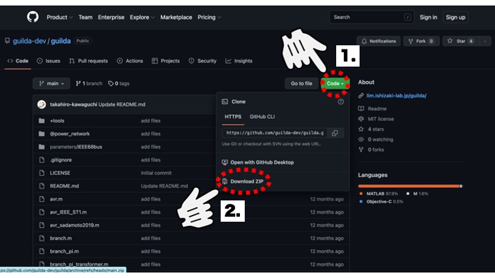
The source code is available to the public on Git. Please use the link from the GUILDA introduction site on the Ishizaki Laboratory's website. You can clone and manage the download from the Git repository. The following images show the procedure to save the files to your local computer as a zip file.

Operation in MATLAB
¶

To open GUILDA in MATLAB:

Extract the source code zip file you have just downloaded, open MATLAB and navigate to the directory.
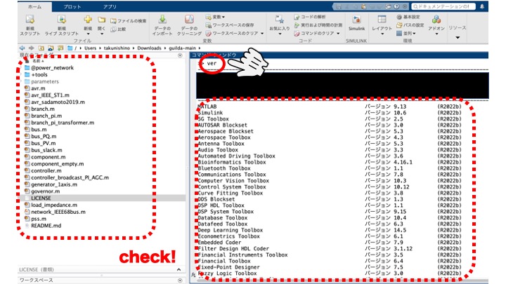
Make sure that the "current folder" window of MATLAB is showing the correct directory. It can be checked by localizing the first folder @power_network, as shown in the image below.
Check if the required toolboxes for GUILDA are installed. To do it write ver in the command window of MATLAB and check if the required toolboxes are installed, these are: Optimization Toolbox, Control System Toolbox, Robust Control Toolbox.

Workflow
¶

In MATLAB it's possible to work one line at the time (via the command window), or several lines at the time (in a script), when performing analysis the latter is recommended.

Recommended workflow:

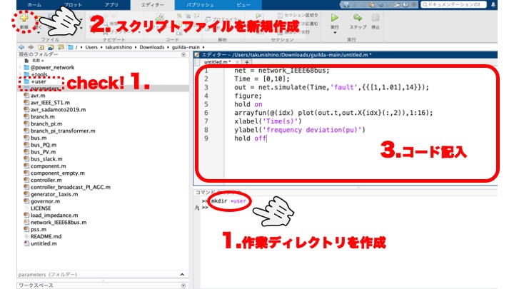
1. Create a working directory: It is recommended that a separated working directory is created, as it will avoid mixing the new created code with the source code. In this example, a new directory named +user is created. The name of the directory can be anything, but make sure to put + at the beginning. This allows the m-files of the source code to be passed through, while also allowing the m-files in the +user folder to be executed.

%Execution command
mkdir +user

2. Create a new script file: Create a new script file by clicking on "New Script" in the upper left corner of the window, which will launch a new file in the editor.

3. Write the Analysis' Code: In the newly created script file, enter the code for the analysis you wish to perform. This documentation and its tutorials mainly focusses on explaining how to write the code in this area. However, for now, just to understand the workflow use the following code as an example; the details are explained in further sections.

%Example code "sample.m"
net = network_IEEE68bus;
Time = [0,10];
out = net.simulate(Time, 'fault', {{[1,1.01],14}});
figure;
hold on;
arrayfun(@(idx) plot(out.t, out.X{idx}(:,2)),1:16);
xlabel('Time [s]')
ylabel('Frequency deviation [pu]')
hold off

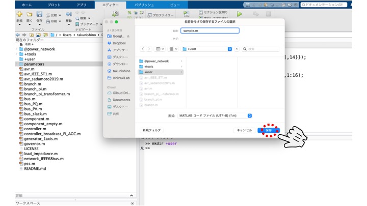
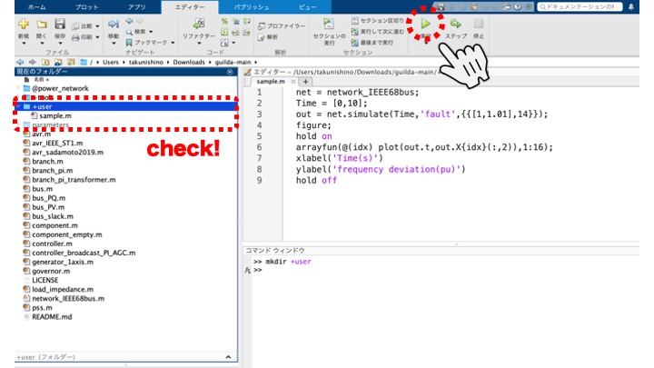
4. Execute: Save the script file you have created and actually execute it. For this example, we will save the script file as sample.m. Note that the newly created file sample.m can be seen now under the +user folder. To execute the code you can press the "Run" button or via the command window, for the latter use the command user.sample.m. This can be use since the user folder has + at the beginning of the directory name. Thus it can be executed as (directory name).(file name).

  %Execution command
  user.sample

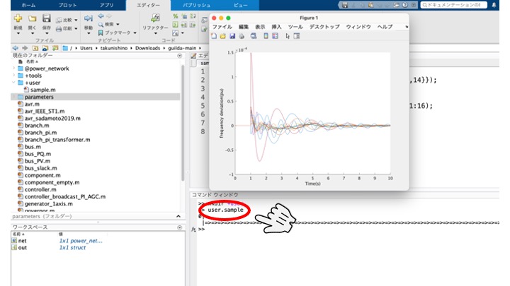
5. Analyze the Results: The analysis performed used the IEEE 68-bus Model, and the plot shows the frequency deviation response of each generator (connected to 1-16th busbar) at [0-10] seconds when a ground fault occurs on the 14th busbar during the timespan of [1-1.01] seconds.

Create a working directory