Simulating

This section explains how to perform the simulations. It explains how to set the simulation conditions and how to read the results.

Contents:

• Simulation Execution Method.
  • Time Argument.
  • Input Argument.
  • Time-Input Relationship.
  • Option Argument.
• Results.
  • Time Variable.
  • State Variable.
  • Voltage and Current Variable.
  • Global Controller State Response Variable.
  • Global Controller Input Variable.
  • Linear Controller State Response Variable.
  • Linear Controller Input Variable.
  • Busbar Variable.
  • Fault Busbar Variable.
  • Admittance Matrix Variable.
  • Solver Variable.
• Auxiliary Tools for Results.
• Simulation Examples

---

Simulation Execution Method

This section explains the function that simulates the power system model, which is defined as a method of the power_network class under the name simulate. The execution method is as follows

%To set the options setting.
out = net.simulate(time,option);

%To set the inputs to the system.
out = net.simulate(time,u,u_idx);

%To set both the option setting, and the inputs to the system.
out = net.simulate(time,u,u_idx,option);

Note: For the data structure of the output result out, please refer to the section Results in the latter half of this page.

From this point on, the arguments of the function simulate are explained.

Time Argument

time = [start, end]

It specifies the time to run the simulation.

For example, if you want to simulate 0-60 seconds, you can specify time=[0,60].

Input Argument

The Input Argument is composed by the arguments u and u_idx, where u is the input to the system, and u_idx is the device number to which the input is applied. By specifying the value of these arguments, a simulation can be performed with inputs to the system. Now u_idx is explained, while u is explained afterwards.

u_idx = [device number]

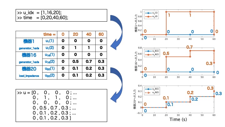
It specifies the device number to which the input is applied. The device number is the number of the busbar connected to the device. As an example here, we consider applying inputs to the devices numbered "1,16,20".

u_idx = [1,16,20];

To set the input values, it is necessary to know the number of ports of the target device and the port number to which the input is given. As for the number of ports, it is obligatory to define a function get_nu in the component class to get the number of input ports, which can be found as follows.

>> for idx = [1,16,20]
      nu = net.a_bus{idx}.component.get_nu;
      disp(['bus',num2str(idx,'%.2d'),':nu=',num2str(nu),'port'])
   end

The port number to which the input is applied must be determined by understanding the respective device model and considering the port number corresponding to the parameter to which you wish to add the input.

For example, in the IEEE 68-bus model, the component 1 and 16 are assigned the generator_1axis class, so the first input port is set to be an input to the field voltage command value and the second input port to the machine torque command value. On the other hand, the component 20 is of the load_impedance class, so the first input port is set to the command value of the multiplier of the real part of the impedance, and the second to the command value of the multiplier of the imaginary part.

Time-Input Relationship

Now, the input to the system (u) is defined. The dimension of u is "the sum of the number of ports of the device to which the input is added "✕" (times) the number of time indices".

In the previous section the argument time was defined as 1✕2 array of the simulation start and end times, but if an input signal is specified, then the argument time becomes the index of the time of the input signal.

In the following image the time-input relationship is depicted by using a zero-order hold.

%Define the arguments time, u, and u_idx as shown above and assign them to the simulate function.
out = net.simulate(time,u,u_idx);

Option Argument

In this section, the possible values of the option argument are explained.

Input Waveform (zero-order hold or first-order hold) (method).

• Zero-Order Hold Input Signal:

option.method = 'zoh';

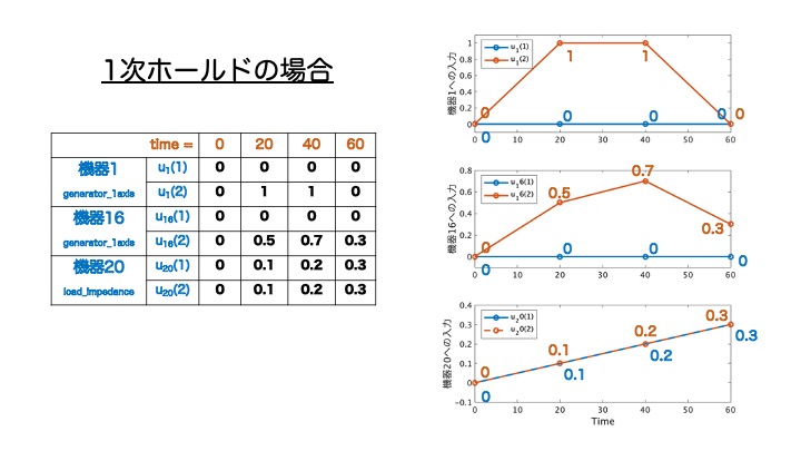
• First-Order Hold Input Signal:

option.method = 'foh';

• Code Example

%Define time, u, and u_idx as shown above and assign them to the simulate function.
%Define the options as 'method' and 'zoh' (zero order hold).
out = net.simulate(time,u,u_idx,'method','zoh');
%Define the options as 'method' and 'foh' (first order hold).
out = net.simulate(time,u,u_idx,'method','foh');

The image below shows an example of a first order hold.

Simulation Linearity (linear).

• Nonlinear Model.

option.linear = false;

• Approximate Linearized Model.

option.linear = true;

Ground Fault (fault).

• No Ground Fault.

option.fault = {};

• Ground Fault - Example 1.

A ground fault occurs on busbar 1 within 1-1.01 sec.

option.fault = {{[1,1.01],1}};

• Ground Fault - Example 2.

In addition to the ground fault in Example 1, another ground fault occurs between 5-5.01 seconds on busbars 2 and 3.

option.fault = {{[1,1.01],1},{[5,5.01],[2,3]}};

• Ground Fault - Example 3.

In addition to the Example 2, a ground fault occurs between 10-10.01 seconds on busbars 4-10.

option.fault = {{[1,1.01],1},{[5,5.01],[2,3]},{[10,10.01],4:10}};

Initial System State Condition (x0_sys).

Initial value of the system state for the equilibrium point.

option.x0_sys = net.x_equilibrium;

Initial Busbar Voltage (V0).

Initial value of each busbar voltage for power flow calculation.

option.V0 = net.V_equilibrium;

• Example: Only the voltage magnitude of busbar 1 is set to be zero \(\small (\lvert V \rvert = 0)\).

option.V0 = net.V_equilibrium;
option.V0(1) = 0;

Initial Busbar Current (I0).

Initial value of each busbar current for power flow calculation.

option.I0 = net.I_equilibrium;

• Example: The current phase of busbar 16 is shifted by \(\small \pi/30\).

option.I0 = net.I_equilibrium;
option.I0(16) = option.I0(16)*(cos(pi/30)+1j*sin(pi/30));

Initial Local Controller State (x0_con_local).

The initial value of the state of each local controller remains at the equilibrium point.

option.x0_con_local = tools.vcellfun(@(c) c.get_x0(), obj.a_controller_local)

Initial Global Controller State (x0_con_global).

The initial value of the state of each global controller remains at the equilibrium point.

option.x0_con_global = tools.vcellfun(@(c) c.get_x0(), obj.a_controller_local)

Error thresholds for Numerical Integration (AbsTol, RelTol).

Minimal required value: \(10^{-8}\)

option.AbsTol = 1e-8;
option.RelTol = 1e-8;

Note: Since GUILDA uses the Solver "ode15s" for numerical integration, please refer to the ODE15S - official documentation for tolerance adjustment.

Simulation Report Output Settings (do_report).

• Generate Simulation Report.

option.do_report = true;

• Don't Generate Simulation Report.

option.do_report = false;

Forced Termination Time (reset_time).

• No Forced Termination Time (default value).

option.reset_time = inf;

• Forced Termination Time - Example: If numerical analysis is not completed within 60 seconds, the analysis is terminated at that point.

option.reset_time = 60;
option.do_retry = false;

Retry Numerical Integration (do_retry).

Once the forced termination time is reached, retry or not the numerical integration.

• Retry (default value).

option.do_retry = true;

• Don't Retry - Example: Please refer to the reset_time condition setting example.

Analysis Results Format (tools).

• Output the Results with Format (default value).

option.tools = false;

• Output the Results without Format.

option.tools = true;

The default is to output the analysis results with format. If this option is set to true, the result will be outputted without format, and just as an instance of the class simulationResult.

Note: If the simulation is planned to be executed several times, it is recommended to use the default value and output the results with format.

Define the Option Argument as a Structure

The function simulate allows you to set detailed simulation conditions by assigning various parameters to the argument option in the form of a structure. The procedure for setting simulation conditions and its example code are as follows.

1. Define the variable option as a structure for setting conditions.
2. Select one of the arguments of option corresponding to the condition you want to set and assign a value to it.
3. Assign the defined optionvariable to the function simulate.

%1. Define the variable option as a structure for setting conditions.
option = struct();

%2. Set initial values for system status.
option.x0_sys = net.x_equilibrium;
%If the frequency deviation (Δω) of the generator in busbar 1 is off by 0.01.
option.x0_sys(2) = option.x0_sys(2)+0.01;

%3.Simulation Execution.
time = [0,60];
out = net.simulate(time,option);

Note: Refer to Network Parameters to see why x0_sys(2) corresponds to the frequency deviation of busbar 1.

While the above explains how to define the variable option as a structure, the function simulate also allows to specify individual conditions directly as arguments. For example, suppose you write the following code

• Define the option Argument as a Structure.

option = struct();

%Initial value of frequency deviation (Δω) of the generator of busbar 1 is deviated 
%from the equilibrium point by 0.01.
option.x0_sys = net.x_equilibrium;
option.x0_sys(2) = option.x0_sys(2)+0.01;

%Ground fault occurs on busbar 5 at 5-5.01s.
option.fault = {{[5,5.01],5}}; 

%Simulation time of 0-10 s.
out = net.simulate([0,10],option);

• Define the option Argument directly in the simulate Function.

Alternatively, the above simulation conditions can also be written as follows

option = struct();

%Initial value of frequency deviation (Δω) of the generator of busbar 1 is deviated 
%from the equilibrium point by 0.01.
x0 = net.x_equilibrium;
x0(2) = x0(2)+0.01;

%Simulation time of 0-10 s with a ground fault that occurs on busbar 5 at 5-5.01s.
out = net.simulate([0,10],'x0_sys',x0,'fault',{{[5,5.01],5}});

Note: When assigning the option argument directly in the simulate function, the arguments are included in the order net.simulate(...'option', 'value',...).

---

Results

This section explains how to read the data in the output result (out).

In the following image an example is presented with the intention to explain its results (out).

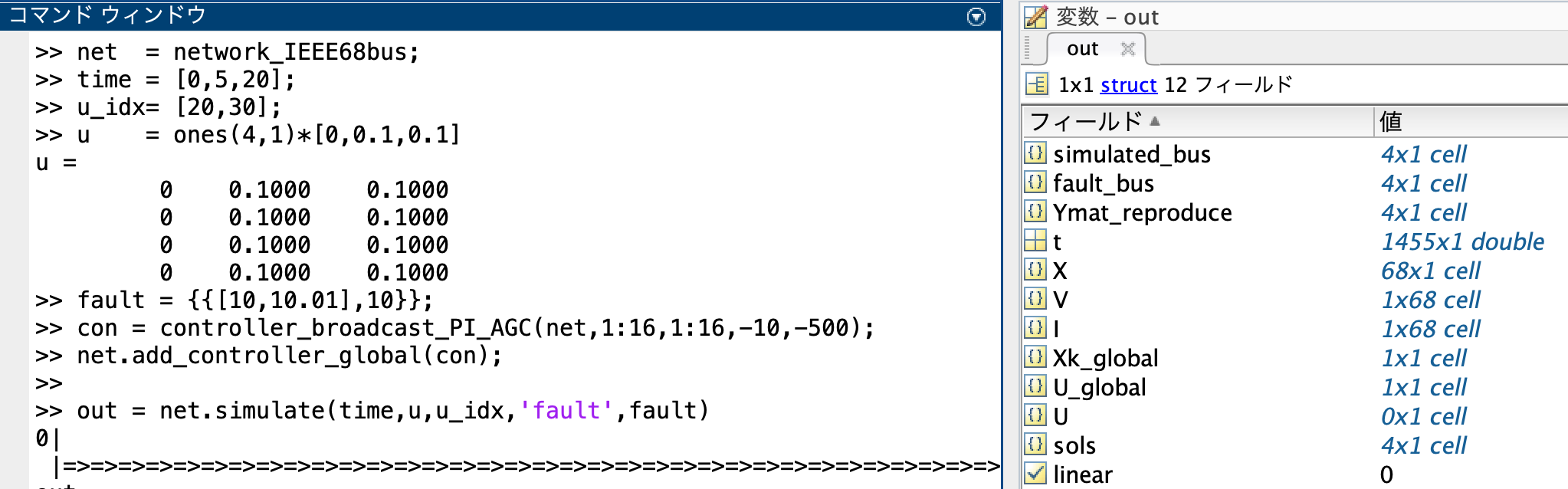
Simulation Example

%The IEEE 68-bus model is defined as the power network.
net = network_IEEE68bus;
%The time-input relationship is stablished
time = [0,5,20];
u_idx = [20,30];
u = ones(4,1)*[0,0.1,0.1]
%The fault on busbar 10 at 10-10.01 is set.
fault = {{[10,10.01],10}};
%An AGC global controller is added to all busbars.
con = controller_broadcast_PI_AGC(net,1:16,1:16,-10,-500);
net.add_controller_global(con);
%The simulation run is stablished.
out=net.simulate(time,u,u_idx,'fault',fault)

Time Field (t)

This field represents the sampling time of the simulation.

It contains an array of "number of samplings", which is used in all the other fields (X,V,I,Xk_global,U_global,U).

Current Example: There are 1455 samplings

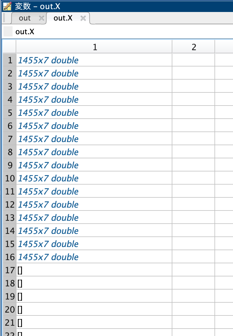
State Field (X)

This field contains the response data of the status of the devices connected to each bus bar.

out.X is a cell array in which each cell corresponds to one device at a time.

The dimension of the numeric array is "number of samplings" ✕ "number of device states".

Current Example: Since the IEEE 68-bus model is used, the busbars 1-16 have a synchronous generator (generator_1axis) with 7 states. Thus, the dimension of the numeric array is 1455 ✕ 7. From the busbar 17th only loads are attachd (load_impedance), which don't have states.

It is possible to call the data of an specific state of a device, for example, the second state of the device connected to busbar 4.

plot(out.t,out.X{4}(:,2))

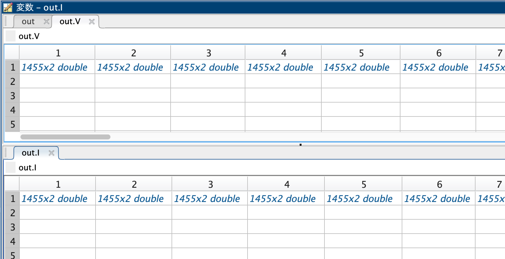
Voltage and Current Fields (V, I)

These fields contain the responses of the voltage and current of the busbars, respectively.

Just like the state field (out.X), the voltage and current fields also are a cell array of the same size as the number of busbars in the system model.

Each cell contains a numeric array with "number of samplings" ✕ 2 (Real Part, Imaginary Part).

Current Example: Each field (i.e., Voltage and Current), have 68 cells (busbars), and each cell has the time response (1455 samplings) of the real part and imaginary part.

It is possible to call the data of an busbar, for example, to plot the magnitude of the voltage and current on busbar 10 during time 10-10.1s (a fault occurs during this time in this bus, thus the expected behaviour is \(\small \lvert V \rvert \to 0; \lvert I \rvert \to \infty\)).

%Read the voltage of busbar 10.
V10 = out.V{10}(:,1) + 1j* out.V{10}(:,2);
%Read the current of busbar 10.
I10 = out.I{10}(:,1) + 1j* out.I{10}(:,2);
%Plot the absolute value of the voltage and current of busbar 10.
plot(out.t,abs(V10),out.t,abs(I10),'LineWidth',2)
legend({'$|V|$','$|I|$'},'Interpreter','latex')
xlabel('Time [s]')
ylabel('Magnitude [p.u.]')

Global Controller State Response Field (Xk_global)

This field contains the global controller state response.

Current Example: In this case, the power system with one global controller added was used in the analysis. Thus Xk_global is a 1✕1 array of cells. The controller class controller_broadcast_PI_AGC has only one state, so the data stored in out.Xk_global{1} is a numeric array with "number of samples".

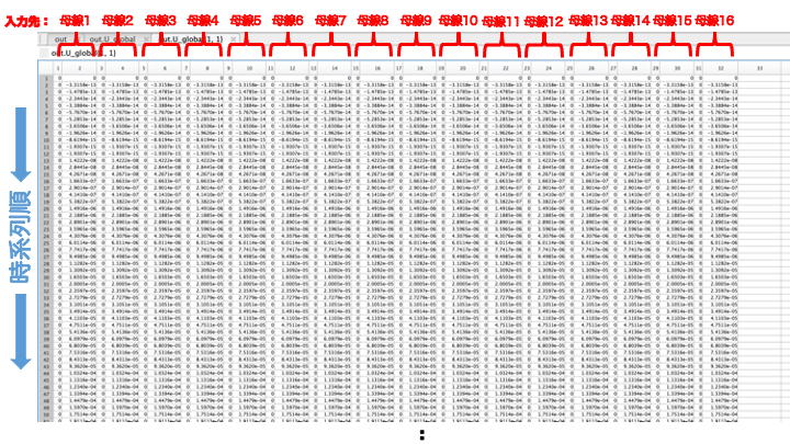
Global Controller Input Field (U_global)

This field contains the response of the input value from the global controller. Like out.Xk_global, this field is also a cell array with the same dimension as the number of controllers attached to the power system under analysis.

Current Example: The controller added in this example is an AGC controller (reads the frequency deviation of the devices in busbars 1 through 16 and gives a command value to the Mechanical Power (Pmech) port of component (added to busbars 1 through 16) to balance the supply and demand of the entire system). In this case, the controller adds inputs to 16 Generators (generator_1axis) with 2 input ports each; thus, it has 2*16 = 32 outputs. Therefore, the data in out.U_gloobal{1} shows "1455 ✕ 32 double".

The correspondence between the input ports and the response data for each device is shown in the figure below, since the devices are specified in ascending order, 1:16, as shown in the code below.

con = controller_broadcast_PI_AGC(net,1:16,1:16,-10,-500);

Each cell is a 2-dimensional array of numbers. The row direction is the chronological order (samples). The column direction follows the input port order.

Current Example: Although the image is small, the first column is all 0 for each cell (i.e., each busbar with a generator). This is because the first input port of the Generators (generator_1axis) is the Field Voltage (Vfield) and the second port is the Mechanical Power (Pmech). The AGC controlle only gives command values to the Mechanical Power (Pmech).

Linear Controller State Response Field (U)

This field contains the local controller state response.

The data is read in the same way as in the global controller state response field (U_global).

Current Example: No local controller is added, so the cell array is empty.

Linear Controller Input Field (linear)

This field is an index indicating whether the simulation was nonlinear or with an approximate linearization.

• Nonlinear: out.linear = 0.

• Approximate Linearization: out.linear = 1

---

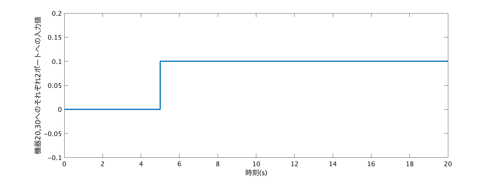
Internal Processes to Consinder

Before describing the data the four remaining fields, a brief description of the processing taking place inside the function simulate is pertinent.

During the numerical analysis, there is usually a point where it becomes discontinuous. For example, when a discontinuous input is given, or when the conditions are discontinuous (e.g., ground fault: the voltage suddenly drops to zero).

In these cases, the solver separates the analysis in two segments, divided by the discontinous point. This means that one solver is dedicated to the first segment of the problem (before the discontuinity), and a new solver is dedicated for the second segment (after the discontinuity). The solver for the second segment starts with the value to which the discontinuity element is applied.

Current Example: The input signal of the current example is shown in the following figure. Furthermore, an ground fault occurs between 10 and 10.01 seconds. Thus, in total there are three discontinuous parts: 1. "The 5-second mark where the input value changes,". 2. "The 10-second mark where the ground fault occurs". 3."The 10.01-second mark where the ground fault ends". Therefore, the numerical analysis is divided into four segments: [0s to 5s], [5s to 10s], [10s to 10.01s], [10.01s to 20s].

With this in mind, the explanation of the remaining fields can be retaken.

---

Busbar Field

For each segment of the analysis: This field stores the index of the components being analyzed.

Note: The busbars with component_empty connected are effectively treated as busbars to which no devices are connected (i.e., non-unit busbars).

Fault Busbar Field

For each segment of the analysis: This field stores the cell array classification of the index of the busbar where the ground fault occurs.

Admittance Matrix Variable

For each segment of the analysis: This field stores in a cell array the generated Admittance Matrix for each segment.

Solver Field

For each segment of the analysis: This field stores in a cell array the solvers running in each segment.

---

Auxiliary Tools for Results (tools)

Finally, this section corresponds to the case when option.tools = true; is used to set simulation conditions.

In addition to the fields described above, the following fields will be newly generated.

• Vabs: Voltage Magnitude \(\small (\lvert V \rvert)\).
• Vangle: Voltage Phase Angle \(\small (\angle V)\).
• Iabs: Current Magnitude \(\small (\lvert I \rvert)\).
• Iangle: Current Phase Angle \(\small (\angle I)\).
• P: Active Power \(\small (P)\).
• Q: Reactive Power \(\small (Q)\).

These fields can be obtained from the data in out.V and out.I, so they are redundant. Therefore, from the standpoint of capacity, these fields may be considered unnecessary. However, this simulationResult class is implemented to serve as an aid in understanding the contents of the output results.

When executed, the following display will appear.

Show "how to use?" (y/n):
%Type `y` and "enter" to display.

Example - Command Input

>> out = net.simulate([0,10],'fault',{{[1,1.01],3}},'tools',true)
0|                                                            |10
 |=>=>=>=>=>=>=>=>=>=>=>=>=>=>=>=>=>=>=>=>=>=>=>=>=>=>=>=>=>=>|

==================================
  Auxiliary tools for outputting simulation results
      SimulationResult Class
==================================

Show usage?(y/n)：

Note that this class can be executed in two ways: 1. By command input (previous example), and 2. By UI Operation.

Example - UI Operation

>> out.UIplot

---

Simulation - Examples

The following page contains examples of handling the simulating functions explained in this page.

Simulation - Examples